Plotting Recipes
ISA.jl includes several plotting Recipes. Recipes are a way of defining visualizations in packages and code, without having to depend on Plots. The functionality relies on RecipesBase, a super lightweight but powerful package which allows users to create advanced plotting logic without Plots.
Two basic visualization type are included in ISA.jl. 1) An Argand Diagram is a geometric representation of a complex number. We provided a way that allows users to visualize AM-FM components using the pre-defined plotting recipes to plot an Argand diagram as follows. First, define a canonical triplet, then call plot() from Plots.jl along with a time range. 2) An Instantaneous Spectrum allows visualization of multiple aspects of the signal model simultaneously, including both magnitude and phase of each signal component. While it may take some time to become comfortable with the 3D visualization, we believe it has significant advantages in terms of interpretability over other time-frequency visualizations.
Setup
After including the Plots.jl package (i.e. using Plots), data types defined in ISA.jl can be plotted by simply calling plot(type) and the corresponding plot recipe will generate the appropriate plot with the default parameters.
Users need to install the Plots.jl package into their system before calling it for the first time. Plots.jl can be installed by typing ]add Plots.
Parameter Options
Below illustrates the use a plotting recipe using default parameters.
using ISA, Plots
𝐶₀ = AMFMtriplet(t->10t,t->25cos(t)+50,0.0)
ψ₀ = AMFMcomp(𝐶₀)
plot(ψ₀, timeaxis=0.0:0.001:3.0)
Plot recipes include default plotting parameters that should be suitable for most cases. However, users can change these parameters as needed.
The following is a list of some of the default parameters used in ISA plot recipes.
| Parameter | Default Value |
|---|---|
| xguide | "time(s)" |
| yguide | "imag" |
| zguide | "real" |
| ymirror | true |
| background_color | first element of colormap |
| foreground_color | :white |
| ymirror | true |
| legend | false |
| framestyle | :origin |
Time-Axis
Below gives an example of setting a custom time-axis range.
plot(ψ₀; timeaxis=0.0:0.001:10.0)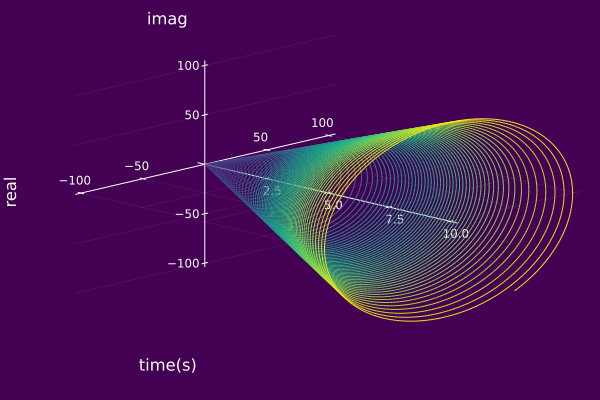
Camera Position
Below gives an example of setting a custom camera position.
plot(ψ₀, timeaxis=0.0:0.001:3.0, camera=(20,50))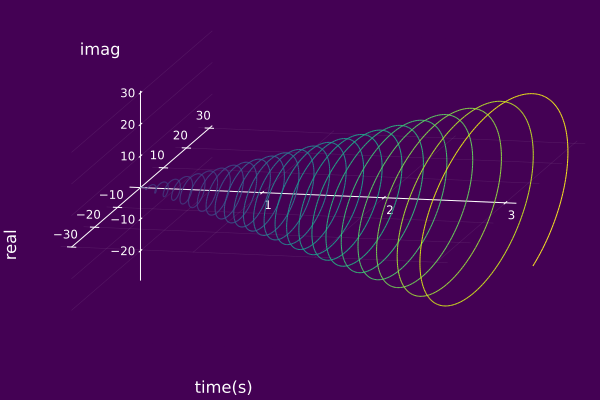
Labels
Below is an example of modifying the axis label and location.
plot(ψ₀, timeaxis=0.0:0.001:3.0,
     yguide="imaginary", ymirror=false)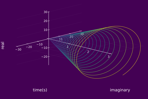
Margins
Depending on the view, you may want to adjust margin sizes.
using ISA, Plots
𝐶₀ = AMFMtriplet(t->exp(-t^2/5),t->200.0,0.0)
𝐶₁ = AMFMtriplet(t->1.0,t->100*t,0.1)
𝐶₂ = AMFMtriplet(t->0.8*cos(11t),t->100 + 70.5*sin(5t),π)
𝑆 = compSet([𝐶₀,𝐶₁,𝐶₂])
plot(𝑆,timeaxis=0.0:0.001:3.0,view="TF",
     left_margin=15Plots.mm, margin=5Plots.mm)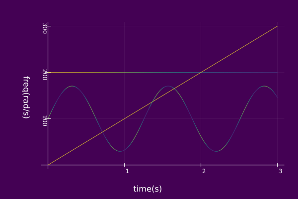
Predefined Views
By default, the plot() function will show a 3D plot. However, the parameter view can be used to 2D plot orthogonal projections of the 3D plot.
Argand Diagram Views
| View | Description |
|---|---|
| default | 3D Argand Diagram |
| TR | time-real plane |
| TI | time-imaginary plane |
| RI | real-imaginary plane |
An example of displaying the default 3D view associated with an AMFMcomp is given below.
using ISA, Plots
ψ₀ = AMFMcomp(t->10t,t->25cos(t)+50,0.0)
plot(ψ₀, timeaxis=0.0:0.001:3.0)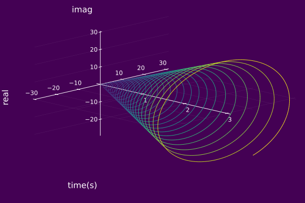
An example of displaying the time-real plane associated with an AMFMcomp is given below.
plot(ψ₀, view="TR", timeaxis=0.0:0.001:3.0,
     left_margin=15Plots.mm, margin=5Plots.mm)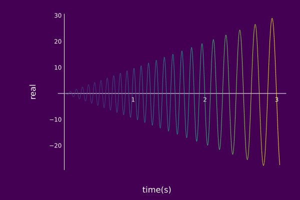
An example of displaying the time-imaginary plane associated with an AMFMcomp is given below.
plot(ψ₀, view="TI", timeaxis=0.0:0.001:3.0,
     left_margin=15Plots.mm, margin=5Plots.mm)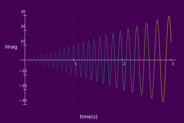
An example of displaying the real-imaginary plane associated with an AMFMcomp is given below.
plot(ψ₀, view="RI", timeaxis=0.0:0.001:3.0,
     left_margin=15Plots.mm, margin=5Plots.mm)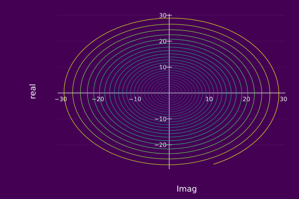
Instantaneous Spectrum Views
| View | Description |
|---|---|
| default | 3D Instantaneous Spectrum |
| TF | time-frequency plane |
| TR | time-real plane |
| FR | frequency-real plane |
An example of displaying the default 3D view associated with an compSet is given below.
𝐶₀ = AMFMtriplet(t->0.2+0.8cos(11t), t->200.0, 0.0)
𝐶₁ = AMFMtriplet(t->exp(-abs(t/3)), t->100t, 0.1)
𝐶₂ = AMFMtriplet(t->𝒩ᵤ(t; μ=1.5, σ=1.0), t->150 + 125sin(5t), π)
𝐶₃ = AMFMtriplet(t->u(t-1.725)-u(t-2.475), t->50, 0.0)
𝑆 = compSet([𝐶₀,𝐶₁,𝐶₂,𝐶₃])
plot(𝑆; timeaxis=0.0:0.001:3.0)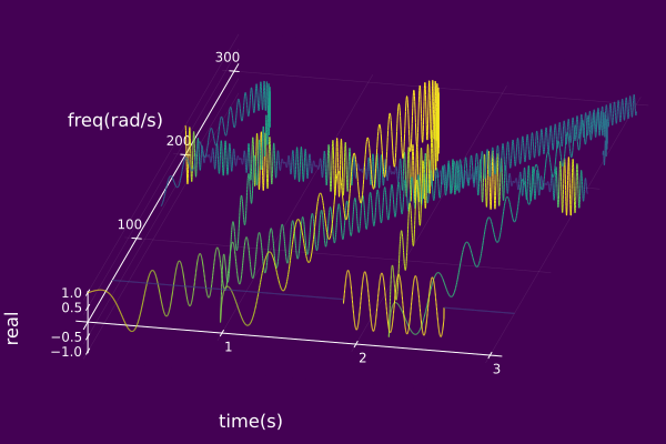
An example of displaying the time-frequency plane associated with an compSet is given below.
plot(𝑆,view="TF", timeaxis=0.0:0.001:3.0,
     left_margin=15Plots.mm, margin=5Plots.mm)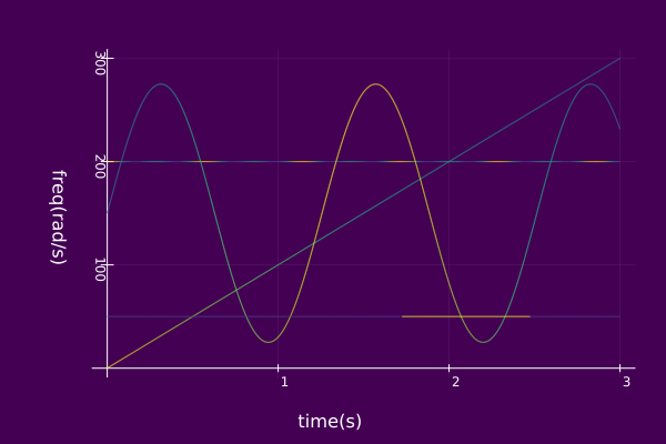
An example of displaying the time-real plane associated with an compSet is given below.
plot(𝑆,view="TR", timeaxis=0.0:0.001:3.0,
     left_margin=15Plots.mm, margin=5Plots.mm)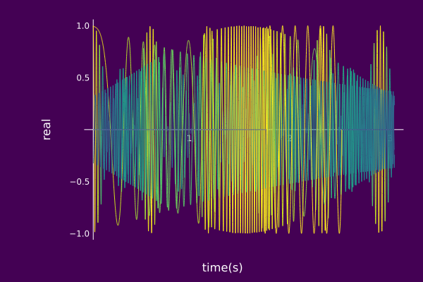
An example of displaying the frequency-real plane associated with an compSet is given below.
plot(𝑆,view="FR", timeaxis=0.0:0.001:3.0,
     left_margin=15Plots.mm, margin=5Plots.mm)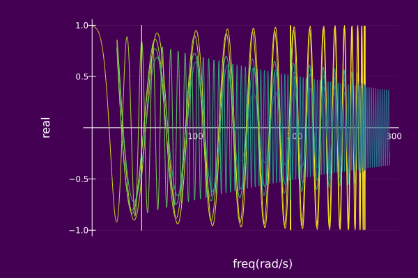
Real Projection
Optionally, the real part of $z(t)$, the real superposition of the components
can be orthogonally projected along the time-axis.
Below is an example of enabling the real projection
using ISA, Plots
𝐶₀ = AMFMtriplet(t->0.2+0.8cos(11t), t->200.0, 0.0)
𝐶₁ = AMFMtriplet(t->exp(-t^2),t->100.0,0.0)
𝑆 = compSet([𝐶₀,𝐶₁])
plot(𝑆,realProj=true)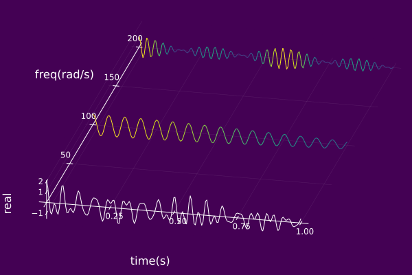
Colormaps
To avoid the perceptual problems associated with many colormaps (Borland and Taylor, 2007; Liu and Heer, 2018), we have utilized two perceptually motivated colormaps in our visualizations. Namely, cubeyf and viridis [default].
An example of using the default colormap (viridis).
using ISA, Plots
ψ₀ = AMFMcomp(t->t,t->25cos(t)+50,0.0)
plot(ψ₀, timeaxis=0.0:0.001:3.0)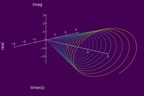
An example of changing the colormap to cubeYF.
plot(ψ₀, timeaxis=0.0:0.001:3.0, colorMap="cubeYF")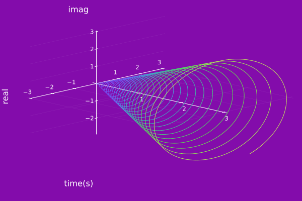
Optionally, users can provide their own customized colormap as a Vector{RGB{Float64}} with 256 element.
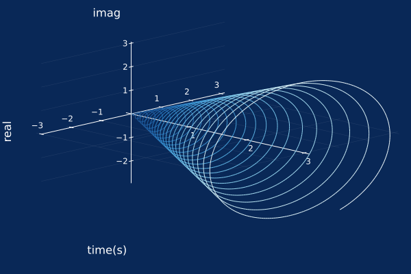
Below is an example of changing the colormap to a user generated colormap myColorMap.
myColorMap  = reverse(colormap("Blues",256))
plot(ψ₀, timeaxis=0.0:0.001:3.0, colorMap = myColorMap)