Consider a component set consisting of a set of harmonically related SHCs
S≜{⋯,C−1,C0,C1,⋯}, Ck={ak,kω0,ϕk00}, k=0,±1,±2,…,±∞. As a result, the components are of the form
ψk(t;Ck00)=akej(kω0t+ϕk) and the AM–FM model corresponding to this set is a Fourier Series
z(t)=k=−∞∑∞akej(kω0t+ϕk). The AM–FM model corresponding to a partial sum (over k) of a Fourier series
z(t)=k=−K∑Kakej(kω0t+ϕk) can be visualized. Additionally, the 3D IS corresponding to partial sum (over k)
S(t,ω,s;S)=2πk=−K∑Kψk(t;Ck00)2δ(ω−ωk,s−sk(t)00) and the 2D IS corresponding to partial sum (over k) (i.e. time-frequency plane)
S(t,ω;S)=2πk=−K∑Kψk(t;Ck00)δ(00ω−ωk00) can also be visualized.
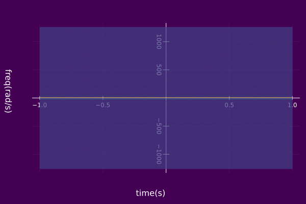
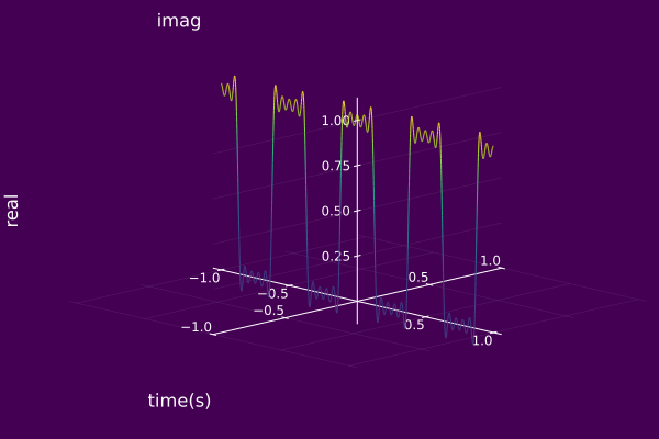
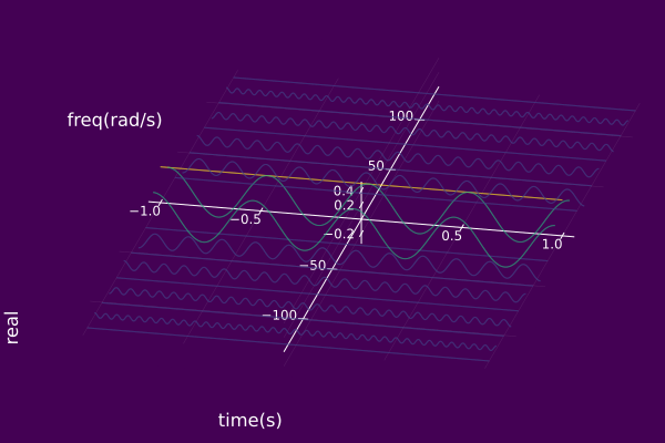
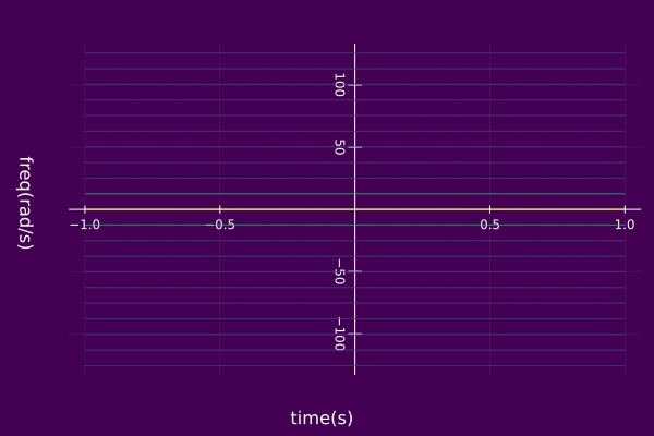
Consider a signal z(t) which consists of a Dirac delta impulse train with fundamental period T.
z(t)=k=−∞∑∞δ(t−kT) We can represent this signal with a component set consisting of a set of harmonically related SHCs
S={⋯,C−1,C0,C1,⋯}, Ck={ak,kω0,ϕk00}, k=0,±1,±2,… where
ak=abs(1/T) and ϕk=arg(1/T). For a this choice of parameters of the component set, we have the following Argand Diagram for z(t;S), 3D IS S(t,ω,s;S), and 2D IS S(t,ω;S). Keep in mind, we are only considering a finite number of components k=0,±1,±2,…,K not k=0,±1,±2,…,±∞.
using ISA, Plots
T = 0.5
aₖ(k) = 1/T
kInds = -10:10
𝑆 = fourierSeries(T, aₖ, kInds)
z = AMFMmodel(𝑆)
plot(z; timeaxis=-1.0:0.001:1.0, ylims=(-1.0,1.0))
using ISA, Plots
T = 0.5
aₖ(k) = 1/T
kInds = -10:10
𝑆 = fourierSeries(T, aₖ, kInds)
z = AMFMmodel(𝑆)
plot(𝑆, timeaxis=-1.0:0.001:1.0)
using ISA, Plots
T = 0.5
aₖ(k) = 1/T
kInds = -10:10
𝑆 = fourierSeries(T, aₖ, kInds)
z = AMFMmodel(𝑆)
plot(𝑆, timeaxis=-1.0:0.001:1.0, view="TF",
     left_margin=15Plots.mm, margin=5Plots.mm)
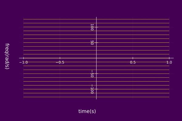
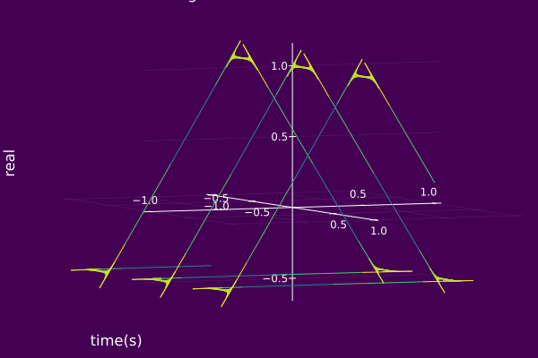
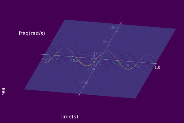
Consider a signal z(t) which consists of a periodic square wave with a 50% duty cycle where one period T is defined by
z(t)={1,0,∣t∣<T/4T/4<∣t∣<T/2. We can represent this signal with a component set consisting of a set of harmonically related SHCs
S={⋯,C−1,C0,C1,⋯}, Ck={ak,kω0,ϕk00}, k=0,±1,±2,… where
ak=abs(kπsin(kπ/2)) and ϕk=arg(kπsin(kπ/2)). For a this choice of parameters of the component set, we have the following Argand Diagram for z(t;S), 3D IS S(t,ω,s;S), and 2D IS S(t,ω;S). Keep in mind, we are only considering a finite number of components k=0,±1,±2,…,K not k=0,±1,±2,…,±∞.
using ISA, Plots
T = 0.5
aₖ(k) = ifelse( k==0, 1/2, sin(k*π/2)/(k*π) )
kInds = -10:10
𝑆 = fourierSeries(T, aₖ, kInds)
z = AMFMmodel(𝑆)
plot(z; timeaxis=-1.0:0.001:1.0, ylims=(-1.0,1.0))
using ISA, Plots
T = 0.5
aₖ(k) = ifelse( k==0, 1/2, sin(k*π/2)/(k*π) )
kInds = -10:10
𝑆 = fourierSeries(T, aₖ, kInds)
z = AMFMmodel(𝑆)
plot(𝑆, timeaxis=-1.0:0.001:1.0)
using ISA, Plots
T = 0.5
aₖ(k) = ifelse( k==0, 1/2, sin(k*π/2)/(k*π) )
kInds = -10:10
𝑆 = fourierSeries(T, aₖ, kInds)
z = AMFMmodel(𝑆)
plot(𝑆, timeaxis=-1.0:0.001:1.0, view="TF",
     left_margin=15Plots.mm, margin=5Plots.mm)
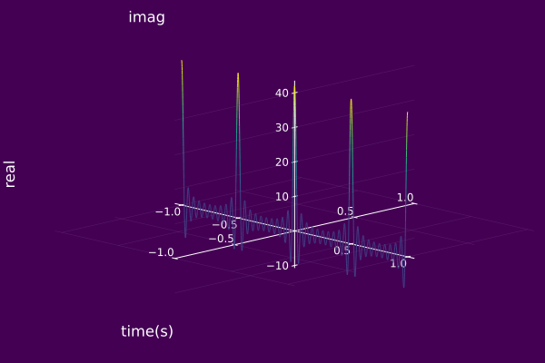
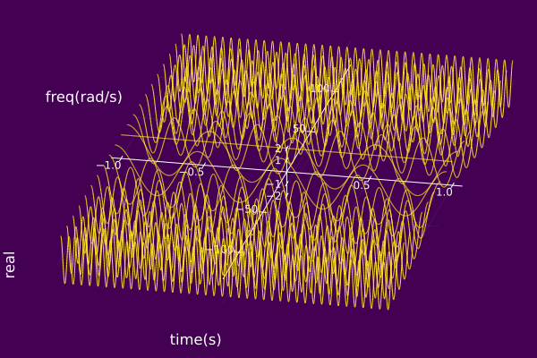
Consider a signal z(t) which consists of a the periodic square wave (fundamental period T) with a 50% duty cycle where one period is defined by
z(t)=⎩⎪⎪⎨⎪⎪⎧1,ej2π/3,ej4π/3,0<t<T/3T/3<t<2T/32T/3<t<T. We can represent this signal with component set consisting of a set of harmonically related SHCs
S={⋯,C−1,C0,C1,⋯}, Ck={ak,kω0,ϕk00}, k=0,±1,±2,… where
ak=abs(jk2π1−e−jk2π/3−ej2π/3e−jk4π/3+ej2π/3e−jk2π/3−ej4π3e−jk2π+ej4π/3e−jk4π/3) and ϕk=arg(jk2π1−e−jk2π/3−ej2π/3e−jk4π/3+ej2π/3e−jk2π/3−ej4π3e−jk2π+ej4π/3e−jk4π/3). For a this choice of parameters of the component set, we have the following Argand Diagram for z(t;S), 3D IS S(t,ω,s;S), and 2D IS S(t,ω;S). Keep in mind, we are only considering a finite number of components k=0,±1,±2,…,K not k=0,±1,±2,…,±∞.
using ISA, Plots
T = 0.75
j=im
aₖ(k) = ifelse( k==0, 0, (1-exp(-j*k*2π/3)-exp(j*2π/3)*
exp(-j*k*4π/3)+exp(j*2π/3)*exp(-j*k*2π/3)-exp(j*4π/3)*
exp(-j*k*2π)+exp(j*4π/3)*exp(-j*k*4π/3))/(j*k*2π) )

kInds = -150:150
𝑆 = fourierSeries(T, aₖ, kInds)
z = AMFMmodel(𝑆)
plot(z; timeaxis=-1.0:0.001:1.0, camera=(60,15))
using ISA, Plots
T = 0.75
j=im
aₖ(k) = ifelse( k==0, 0, (1-exp(-j*k*2π/3)-exp(j*2π/3)*
exp(-j*k*4π/3)+exp(j*2π/3)*exp(-j*k*2π/3)-exp(j*4π/3)*
exp(-j*k*2π)+exp(j*4π/3)*exp(-j*k*4π/3))/(j*k*2π) )

kInds = -150:150
𝑆 = fourierSeries(T, aₖ, kInds)
z = AMFMmodel(𝑆)
plot(𝑆, timeaxis=-1.0:0.001:1.0)
using ISA, Plots
T = 0.75
j=im
aₖ(k) = ifelse( k==0, 0, (1-exp(-j*k*2π/3)-exp(j*2π/3)*
exp(-j*k*4π/3)+exp(j*2π/3)*exp(-j*k*2π/3)-exp(j*4π/3)*
exp(-j*k*2π)+exp(j*4π/3)*exp(-j*k*4π/3))/(j*k*2π) )

kInds = -150:150
𝑆 = fourierSeries(T, aₖ, kInds)
z = AMFMmodel(𝑆)
plot(𝑆, timeaxis=-1.0:0.001:1.0)
plot(𝑆, timeaxis=-1.0:0.001:1.0, view="TF",
     left_margin=15Plots.mm, margin=5Plots.mm)